FEA Modelling Services

FEA is generally preferred for modeling magnets because it is said to be better at modeling non-linear problems (e.g. magnetic saturation of mild steel). BEA however is better at modeling fields in free space and does not require boundary air boxes. Hybrid solvers combine the best of both but require very powerful computers to give reasonable solve times. 2D solvers are standard and can model axi-symmetrical models. They can estimate simple 3D by giving the entire model the same depth (otherwise the depth may be regarded as either very small or infinite). True 3D solvers allow varying depths and varying locations for components but again take much longer to solve and require high performance computers for reasonable solve times. Solvers can be static (i.e. a snap shot in time) or dynamic (i.e. time varying). Dynamic solvers take much longer to solve.

We offer static 2D FEA with axi-symmetric solving capability. It is good practice to understand the entire magnetic model beforehand and to solve based on a worst case scenario(s). There may be occasions where the magnet will demagnetise in the application. Many solvers cannot compensate for this and then model too high a magnetic output. It is possible to interpret the initial results and to then re-program the BH curves to solve again to get more accurate solutions. FEA takes a standard BH curve for not only the magnet material but also the magnetic steels. The real world has variations in output. Again, it is good practice to model with the lowest performance in mind and to accept that real world performance may be better although there is no reason why a range of BH curves could not be solved for if time allowed (e.g. to compensate for batch to batch variations in the magnetic performance). A pessimistic view of FEA and BEA is that it allows a relative performance comparison to be made if modeling variants of a design. However this can still be very cost effective compared to making full size real world assemblies. It should be noted that most FEA and BEA solvers use the Normal curves and, as such, risk not modeling magnets correctly (as it is the Intrinsic curve that is used for demagnetisation effects) e.g. N42 appears the same as N42SH in FEA but the performance would be different between the grades at 140 degrees C. A trained user of FEA / BEA would be able to factor in a compensation is the problem to be solved required it. Very few solvers correctly take demagnetising and temperature effects into account so caution is required.

FEA can be used for modeling almost any magnetic problem. Examples include Halbach Arrays, Loudspeakers, Motors and Generators, Sensors, Pump Couplings and clamp systems. To solve a design, a 2D dxf file can be imported (drawn to scale) and this is then defined in FEA (material properties defined, meshing defined and optimised, solver parameters defined) and then solved (done by the computer). Examples of results that can be obtained (sometimes called post processor analysis) are Magnetic Field Strengths (magnitude and direction for B and H), forces acting on objects (magnitude and direction) and torque acting on objects (magnitude and direction) and can include graphs and pictures. Analysis of the results will allow determination of suitability of the design, identification of areas for improvement and identification of possible demagnetisation.

e-Magnets UK offers static 2D FEA with axi-symmetry as a service to its customers. Where possible it if free or we may ask that a fee is paid which is discounted from any subsequent order as a result of the FEA work. Please contact us for more details.

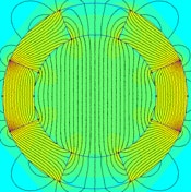
Example FEA Magnetic Field Plot for a Dipole Halbach Array